Filtering With Buffers – SpatialKey Support

⬅ Knowledge Base Home

Filtering with buffers is a powerful way to perform analysis on your datasets. For example, you can set up criteria to show only locations from Dataset A that fall within [x] miles of Dataset B. Now plug your use case in that example…

I want to see prospects within 10 miles of my sales reps
I want to see clients that are farther than 30 miles from my repair shops
I want to see houses for sale within 500 meters of a school
I want to see my insurance policies within 250 meters of terrorism targets
I want to see houses for sale within 500 meters of a golf course
I want to see my insurance policies within 100 feet of the Mississippi river
I want to see my insurance policies within 29 miles of a hurricane track

There are endless possibilities of how to use this analytic capability. The first 4 examples above require buffering around a point dataset, the next 2 examples require buffering around polygons and the last example above requires buffering around a line. Setting up these buffers is the same for all of these different examples so let’s walk through how it is done with an example where we will buffer around polygons.

Setting up a buffer

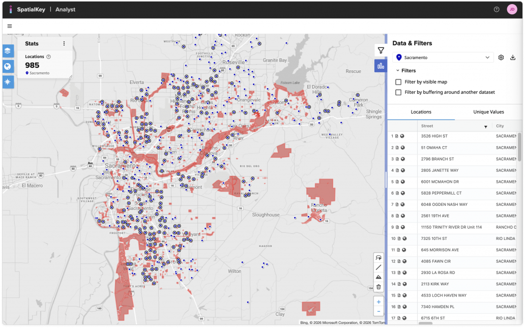
My dataset contains a list of approximately 1,000 homes for sale in the Sacramento area. To help my client narrow down this list to homes they are interested in, we can apply buffers around park boundary data. In the image below, you can see the homes for sale (blue points) and the parks (red boundaries).

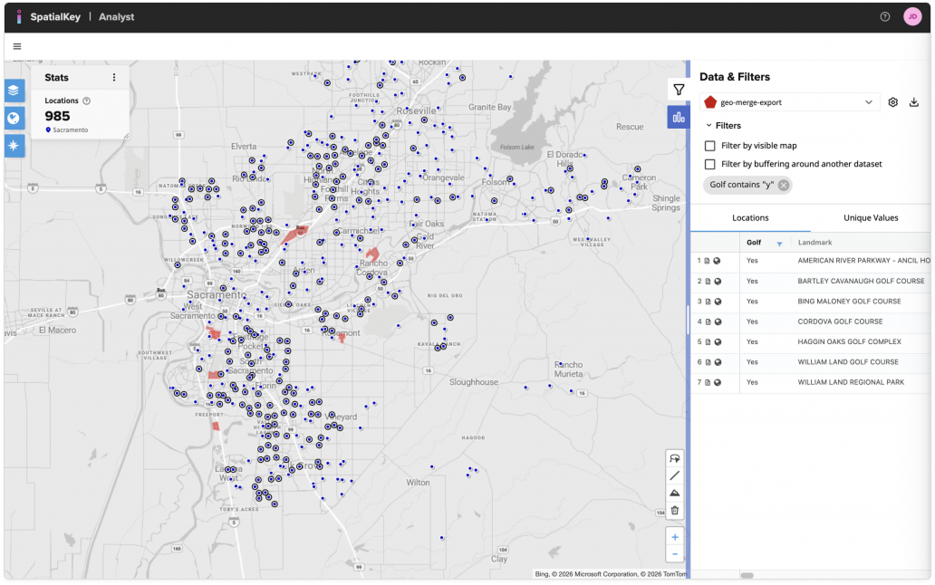
Screenshot of the SpatialKey Analyst web map showing a city‑scale view of Sacramento. Hundreds of blue location markers are displayed across the map, while irregular red shaded areas representing parks covering parts of the city. A stats panel on the left reports 985 locations for Sacramento. On the right, the “Data & Filters” panel shows Sacramento selected with options to filter by visible map or by buffering around another dataset, and a locations table listing street addresses filtered to the map view.

My client is interested in looking at homes within 250 meters of a golf course. We can first apply a filter to limit our park boundary data by golf courses.

Screenshot of the SpatialKey Analyst web map showing a city‑scale view of Sacramento. Blue dots represent homes for sale distributed across the metro area. Red shaded boundaries represent golf course polygons, highlighting their locations within the city. A stats panel on the left reports 985 homes for sale. On the right, the “Data & Filters” panel shows filtering options for the geo‑merged export, and the locations table lists golf course landmarks used to contextualize nearby home listings.

At this point, we could zoom in and visually identify homes that are “close” to open space or golf courses, but it would be more efficient to let SpatialKey perform this analysis for you.

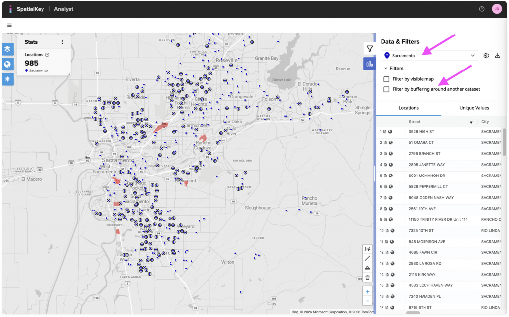
Click on the dataset that you want to filter – in this case, we want to filter the Sacramento locations by buffering around the park boundary data. Select the “Filter by buffering around another dataset” in the Location Report tab on the right side of the map.

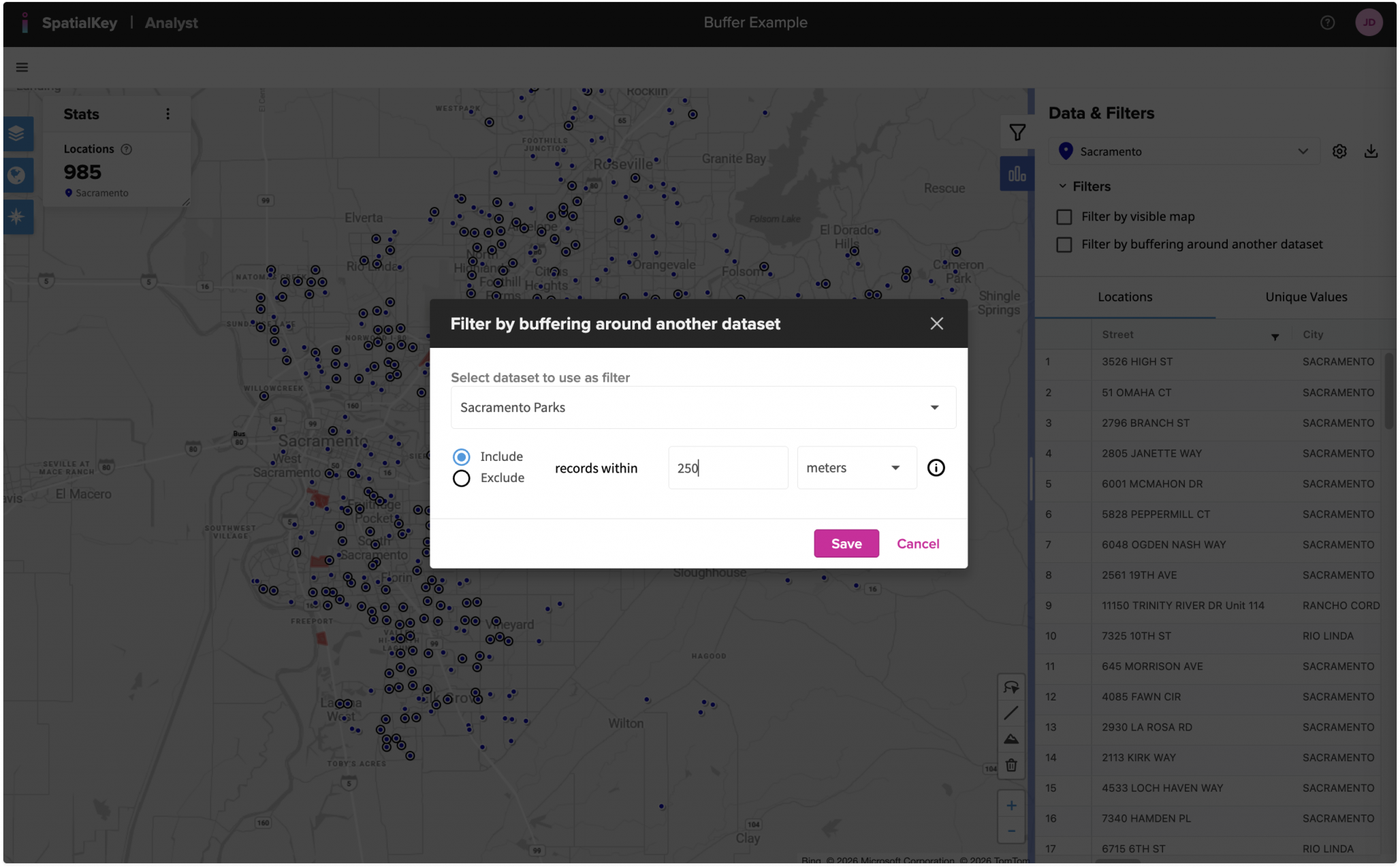
Screenshot of the SpatialKey Analyst web map showing a city‑wide view of Sacramento with blue dots representing homes for sale and red polygon boundaries representing golf courses. In the right‑hand “Data & Filters” panel, the user is prompted to first select a dataset and then choose “Filter by buffering around another dataset,” highlighted by arrows. This filtering option is used to perform a proximity analysis, identifying homes for sale located within 250 meters of a golf course. The map will then display only homes that meet the buffer criteria, and the locations table updates to reflect the filtered results.

Fill out the options on this screen to enable the buffer:

Select which dataset to “Use as filter” – in this example, we only have one other dataset in the dashboard so we’ll select the “Sacramento Parks” dataset
Set to include or exclude records that meet the filter criteria
Set the distance of the buffer
Click to “Save” the filter

In this case we’ll include locations that are within 250 meters of the Sacramento Parks.

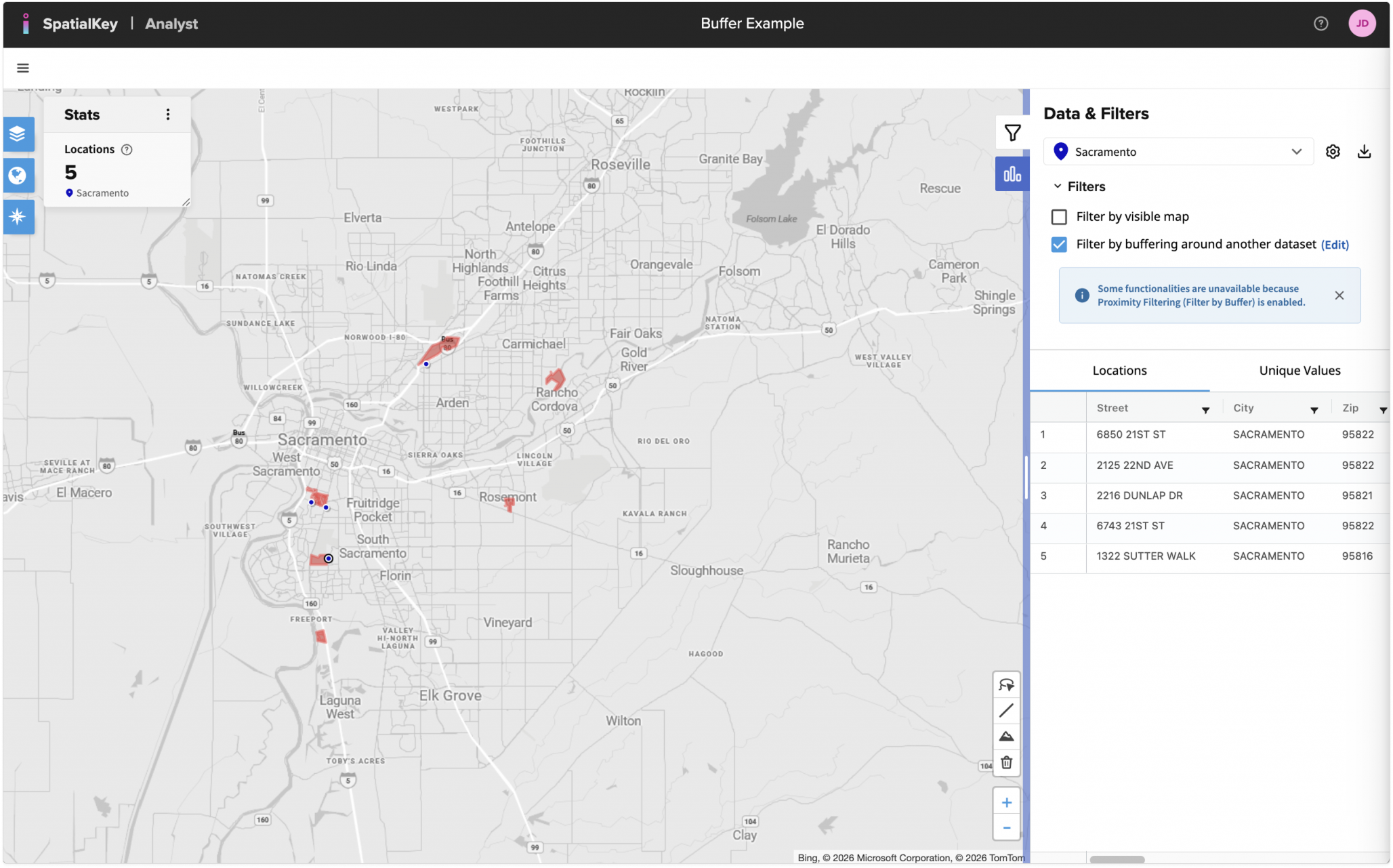
Screenshot of the SpatialKey Analyst web map with a modal titled “Filter by buffering around another dataset” open on top of a Sacramento map. The dialog prompts the user to select a dataset to use as a filter (set to Sacramento Parks) and to include records within 250 meters, with options to include or exclude results. Behind the dialog, blue dots representing homes for sale remain visible on the map, indicating that the buffering settings will filter homes based on proximity to the selected dataset once saved.

You’ll notice that your data has been filtered to show only the 5 homes within 250 meters of the desired park boundaries.

Once you enable filtering by a buffer, your dataset becomes locked. You will see this on the “Data & Filters” tab for the dataset. To change the filter on your locked dataset, you will need to disable the buffer filter first.

Screenshot of the SpatialKey Analyst web map showing buffer analysis results for Sacramento. Blue dots representing homes for sale have been filtered down to five locations that fall within 250 meters of the selected comparison dataset. Red shapes on the map indicate the nearby reference features used in the proximity analysis. In the “Data & Filters” panel, “Filter by buffering around another dataset” is enabled, and the locations table lists the five homes that meet the buffer criteria.

That’s all there is to applying a buffer!

One thing to note, if you are buffering around a shapefile (boundary file) that is too complex, you will see a message when trying to apply a buffer. You can work around this by applying a filter to your dataset before trying to apply a buffer. We did this in the example above by filtering the boundary dataset by golf courses.

Was this helpful?

Yes

Thanks for your feedback!